/*     x(t)   =     A      *      x(t-1)   +  v(t-1)
 * [  x1(t) ] = [ 1 0 .04 0 ] [  x1(t-1) ] + [  wx1 ]
 * [  x2(t) ]   [ 0 1  0 .04] [  x2(t-1) ]   [  wx2 ]
 * [ dx1(t) ]   [ 0 0 .99 0 ] [ dx1(t-1) ]   [ wdx1 ]
 * [ dx2(t) ]   [ 0 0  0 .99] [ dx2(t-1) ]   [ wdx2 ]
 *
 *     y(t)   =     C      *    x(t-1)   +      D       *    u2(t)   +  n(t)
 * [  y1(t) ] = [ 1 0 0 0 ] [  x1(t-1) ] + [ -1  0 0 0 ] [  rx1(t) ] + [ vx1 ]
 * [  y2(t) ]   [ 0 1 0 0 ] [  x2(t-1) ]   [  0 -1 0 0 ] [  rx2(t) ]   [ vx2 ]
 *                          [ dx1(t-1) ]                 [ drx1(t) ]
 *                          [ dx2(t-1) ]                 [ drx2(t) ]
 */
cycle duration: 0.04sec
ball vel decay: 0.99
Particle filter uses SIR algorithm.
I set the segway at unbalanced mode. This is the static ball test setup.

The origin is at the center of the wheels.

Robot's view when I put the ball at (.9, 0).

I collected the result of kalman filter and particle filter when the ball is at (.9, 0) and (2.7, 0) respectively. From the result, it seems KF is better in terms of standard error when the ball is closer. When the ball is far away, PF is better. But we may need more tests to conclude.
| # data | KF mean | KF std | PF mean | PF std | |
(0.9, 0) | 2243 | (0.7488, 0.3392) | (0.0005, 0.0009) | (0.7489, 0.3393) | (0.0018,0.0018) |
(2.7,0) | 7210 | (3.9065,0.3168) | (0.4610,0.2817) | (3.9722,0.2829) | (0.0679,0.3811) |
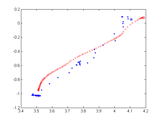
Moving-ball test setup. I kick the ball back and forth between (3.6, 0) and (3.6, -2.7). Note these two points are observed by the segway as (4.20, 0.15) and (3,45, -0.94) in the current setup. I run the test for about 3 minutes (4212 cycles) and record the tracking result of KF and PF.

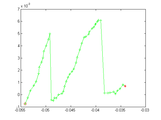
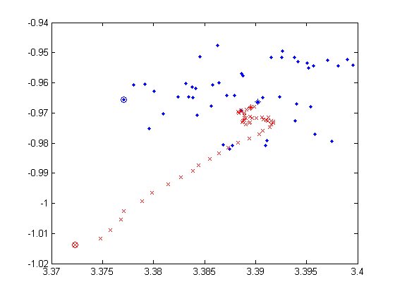
Below are 4 selected predicted trajectory of KF and PF during 100 cycles. In each plot, x/y axis is the predicted x/y relative position of the ball, the blue dot denotes the KF prediction and the red cross represents the PF prediction. And the circle is the starting point, while the star is the ending point. Though we do not know exactly the true value of each intermediate position of the ball, I kick the ball straightly and try to keep it rolling in a straight line (directly from (3.6, 0) to (3.6, -2.7). In each plot, it is obvious that PF prediction is much smoother than that of KF.
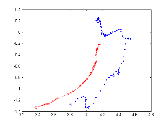

The other new feature of this PF implementation is the velocity estimation. Here are two sets of plot.
The below one is similar to the above 4 but it is during 50 cycles.
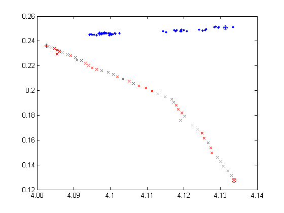
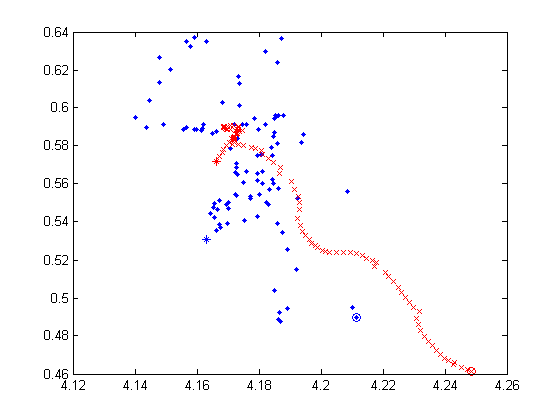
This is the corresponding velocity estimation from PF. x and y axis are predicted v_x, v_y of the ball.
Here is another set.
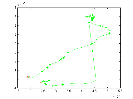
It can be seen that the predicted velocity is quite usable in these two cases.
TODO:
- test: moving robot observes static ball
- test: moving robot observes moving ball
- handle with false positive
- better movement model
- Next: tracking markers and self-localization by PF